Barclay T.Leib – Measuring Financial Time The Magic of Pi

Salepage : Barclay T.Leib – Measuring Financial Time The Magic of Pi
Archive : Barclay T.Leib – Measuring Financial Time The Magic of Pi Digital Download
Delivery : Digital Download Immediately

“This study first published on Sandspring.com on February 25, 2001. It is a long-term examination of cyclical equities market rhythms, although it is already four months old. Size of the file: 106 KB

Barclay T.Leib – Financial Time Measurement The Story of Pi

“This study first published on Sandspring.com on February 25, 2001. It is a long-term examination of cyclical equities market patterns, but it is also little antiquated given that it is four months old. When Mr. Leib’s specified in the article $294.50 Fibonacci gold objective was attained, he suggested to book profits and become short-term neutral gold.”

Michael Alexander does an amazing job dispelling the myth that “the greatest moment to purchase stocks is usually now since equities in the long term always go up” in his new book Stock Cycles (Writers Club Press, iUniverse.com, 2000). Beginning with historical history, he demonstrates that, given the valuation levels at the start of 2000, “there is a 75% risk of negative capital gains return over the following 20 years,” and a “zero percent chance of the S&P 500 returning even 15% over the next five years.”

Given the recent battering of the S&P 500, Alexander appears to have been exceptionally foresighted. It’s a shame that it takes so long for book publishers to turn decent content into final bound form.

In true academic fashion, Alexander then divides equities market activity into two cycles: “monetary” and “real,” each of which can have four fundamental permutations:

1) High real incomes, high inflation

– Market chop that is typically sideways

2) High real incomes with little inflation

– times of market expansion

3) Low real incomes due to low inflation

– times of deflation/depression and bond market booms

4) High inflation and poor real wages

– Equity market stagflationary eras

As a result, while earnings growth in the United States was roughly the same between 1965 and 1982 as it was between 1982 and 1999, Alexander attributes the sideways performance of stocks during the first of these decades to a negative inflationary monetary environment. Markets, on the other hand, thrived in the latter era due to a healthier monetary environment.

Similarly, Alexander contrasts the years 1929-1948 with 1948-1965. He discovers that, while monetary conditions were comparable in both times, actual wages were drastically different. In the first phase, real profits were low, and inflation was low, resulting in a bond bull market rather than a stock bull market. Low inflation mixed with high real incomes produced a powerful bull market in the latter years.

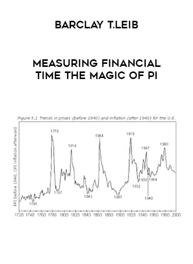
All of this is wonderful and dandy, but Alexander appears to overlook the clear regularity of these periods: each lasts around 17 years. He does remark that the troughs between U.S. inflationary eras are spaced an average of 51 years apart (interestingly, 3 x 17 years), and he includes this beautiful long-term graphic of U.S. pricing trends:

Michael Alexander’s Stock Cycles.

If the usual 51-year inflationary trough pattern continues, 1949 + 51 years = 2000, implying that inflationary tendencies should already be on the rise – which they are. At most, this suggests that equities will replicate their chop performance from 1965 to 1982 as inflation begins to buffet any profit increase. At worst, it means that if profits growth begins to fall on its own (as the newspapers have been reporting on a daily basis recently), a stagflationary collapse is possible.

But first, let’s take a closer look at the 17-year cycle Alexander so deftly mentions but then fails to elaborate on. More specifically, we believe it is a 17.2-year cycle. Why was it 17.2 years? We must begin with the work of Martin Armstrong, who felt he had uncovered a cycle known as the Princeton Economic Confidence Interval of 8.6 years by analyzing the average distance between market panics in the nineteenth and twentieth centuries. He felt that the markets had repeated 8.6 year cycles that built in intensity to generate a long-wave of economic activity lasting 51.6 years.

Now, 8.6 years equates to 3,141 days, which is quite close to the mathematical number of pi (3.14159) multiplied by a thousand. Twice pi multiplied by 1000 equals 6,283 days or 17.2 years.

Remember this equation from elementary school:

2 ** r = a circle’s circumference

Assume that r, or the radius, is equal to a base unit of one. This equation would then be reduced to only 2 *, or the radius of a circle equivalent to the completion of one full cycle in our cognitive process. Isn’t it cool? After all, if notions like calculating the circumference of a circle are valid in the real world of geometry, why shouldn’t they be valid on Wall Street?

As a result, we arrive to the following hypothesis:

Learn How to Measure Financial Time Only $27 for The Magic of Pi – Barclay T.Leib

While the magnitude of up and down price fluctuations in equity markets is clearly governed by the rules of the Fibonacci Golden Ratio.618 (and its reciprocal 1.618) derived from the Fibonacci Number Sequence 1,1,2,3,5,8,13,21…., the duration of economic cycles is governed by cycle 2 * rather than Fibonacci.

What anecdotal evidence supports our belief in the significance of 2 *?

The South Sea Bubble, possibly the most famous panic of all time, occurred in 1720. Prior to then, the worst financial crisis occurred in 1092, when the practice of debasing the precious metal content of currencies resurfaced for the first time since the collapse of the Roman Empire, and interest rates in Britain soared to more than 50% per annum. The time interval between these two occurrences occurs to be 2 ** 100 = 628 years. Isn’t it an odd coincidence?

628 years before that incident, in 464 AD, the Vandals had taken over the Roman Empire and the Anguls had invaded Britain. At the time, the Roman money was in serious decline, resulting in another financial catastrophe.

Bringing our long-term analysis into the modern United States spectrum, exactly thirteen 17.2 year periods transpired as of February 23, 2000 — a date that fell almost exactly between the January 2000 high in the Dow Jones Industrials and the late March high in the NASDAQ and S&P 500.

Another coincidence? Perhaps. But let’s look at the thirteen 17.2-year cycles in between, breaking them down into their twenty-six 8.6-year half-cycles and focusing on the rhythm of inflation vs stock prices. As we continue, we’ll aim to assign a “Alexander classification” to each cycle.

We begin on July 4, 1776 and work our way forward. Not only does 1776 commemorate the beginning of our country, but it also occurs precisely five 17.2-year cycles (86 years) after the first paper money experiment in the United States in 1690. In 1690, the Massachusetts Bay Colony used paper money known as Bills of Credit to pay for a military expedition to Canada during King William’s War. As a result, we do not consider our decision to investigate the rhythm of modern times beginning on July 4, 1776 to be inherently wrong in its arbitrariness.

We’ll try to find a pattern of behavior once we’ve described all of the individual 8.6 year half-cycles inside the 17.2 year overall cycles. Please bear with us while we do some historical research.

The initial 17.2 year cycle

War, inflation, and forgery characterized the early half of this period, which lasted from July 4, 1776 through February 8, 1785. Four Continental Congress dollars equaled one gold dollar in 1778. A year later, the ratio had risen to 100-1. To begin, we will refer to this as an Alexander type 4 high inflation/low real incomes era.

From February 8, 1785 through September 16, 1793: A downturn struck the post-war period when wholesale prices fell between 1784 and 1787. Debtors were increasingly demanding that states print paper money in order to devalue the currency and thereby lessen the debt load by 1786. By 1791, the Netherlands was in the grip of a deflationary panic, which had been aggravated by the failure of land speculator William Deur. British Consols (bonds) were in high demand. Several banks collapsed, leading Secretary of the Treasury Alexander Hamilton to flood the system with cash through the United States Treasury’s purchase of stocks and bonds. The 1791 Panic was the first serious crisis in the post-Revolutionary War United States. We’d categorize the last 8.6 years of this period as an Alexander type 3 period of net low inflation, low earnings….with equities under pressure and foreign bonds heavily bid.

The second 17.2 year cycle

Between September 16, 1793 and April 24, 1802, the Treasury changed the forces of deflation into forces of inflation. Throughout the era, prices grew steadily. The economy grew strongly as well, but this inflation dampened its growth. As a result, equities remained under pressure during these years, which were clearly an Alexander type 1 period of high inflation and high growth, with the two net offsetting each other.

Between April 24, 1802 and November 30, 1810, inflation continued to rise while growth slowed. Another mild Alexander type 4 stagflationary period.

Cycle No. 3 (17.2 years)

From November 30, 1810 to July 7, 1819: Following the War of 1812, deflationary forces returned to the United States, eventually leading to the 1818 Panic when the Second Bank of the United States failed. Manufacturers in the United States have called for higher tariffs to protect their products. Deflation combined with low earnings produced an Alexander type 3 period.

From 7 July 1819 to 12 February 1828: However, during the second 8.6 years of this cycle, the US economy recovered while commodity prices fell, resulting in a period known as the “Era of Good Feelings” and clearly an Alexander Type 2 period.

Cycle No. 4 (17.2 years)

From February 12, 1828 to September 18, 1836, there was relatively low inflation and strong growth in earnings, yielding another 8.6 years of an Alexander Type 2 period.

Sep 18, 1836 – April 26, 1845: Andrew Jackson’s campaign to return U.S. banking to the states succeeded in undermining confidence in the currency. New York banks in May 1837

Many other banks across the country followed suit and stopped redeeming paper money for gold. By the end of 1937, 618 banks had failed, and gold had vanished from circulation. The only money in circulation was private bank currency of dubious value and frequently counterfeit origin. It would take until 1846 for an independent and more stable treasury system to be established. Gold soared in its purchasing power during these years. This was clearly a stagflationary Alexander type 4 period even as other commodity prices slumped.

Fifth 17.2 Year Cycle

April 26, 1845 – December 1, 1853: Large-scale industrial growth arrived with the westward expansion, railroad construction, and the discovery of gold out west. A high growth environment, but with rising inflation leading to an Alexander type 1 mixed period classification.

December 1, 1853 – July 10, 1862: Over-expansion in land and railroad speculation led to a financial panic in 1860, with declining asset prices and inflation, a type 3 Alexander period.

Sixth 17.2 Year Cycle

July 10, 1862 – Feb 14, 1871: The onset of the Civil War and deficit spending by the Treasury to finance the war brought another period of rampant inflation. But the economy was experiencing real growth to produce goods in support of the war. A type 1 Alexander period was the net result, punctuated by a brief gold panic in 1869.

Feb 14, 1871- Sep 22, 1879: After a panic in railroad stocks in 1873, inflation dropped consistently during these years, while real growth in the economy was strong. These were vintage Alexander type 2 boom years.

Seventh 17.2 year Cycle

Sep. 22, 1879 – April 28, 1888: Inflation continued to head lower during these years, and big business and increased industrialization continued to arrive. Stock prices did not advance dramatically, but we would still call these Alexander type 2 years.

April 28, 1888 – Dec 4, 1896: 1888 saw a turn against big business with the introduction of antitrust legislation, and the reversal of excess railroad speculation. Particularly after the Panic of 1893, it became a low growth, low inflation economy – a type 3 Alexander environment.

Eighth 17.2 year Cycle

Dec 4, 1896 – July 12, 1905: 1897 saw the trough in deflation, and American growth and imperialistic pride led us into the Spanish-American War of 1898. Increasing inflation and growth marked this as an Alexander type 1 period.

July 12, 1905 – Feb 17, 1914: Strong inflationary trends and progressive trends in favor of better work conditions for labor made this a poor time to be an equity investor. The panic of 1907 was short-lived and of little consequence, but we’d call this period an Alexander type 4.

Ninth 17.2-year Cycle

Feb 17, 1914 – Sep 24, 1922: War years brought a nice step-up in corporate earnings, but further inflation to finance the war effort, with a break in commodity prices in the latter half of the period. This is perhaps our hardest period to categorize, but we’ll call it overall an Alexander type 1 environment.

Sep 24, 1922 – May 2, 1931: Low inflation plus high real U.S. economic growth led to an equity market boom that despite the severity of the Oct 1929 market plunge, truly did not reverse until after May 1931. This was an Alexander type 2 boom environment.

Tenth 17.2 year Cycle

May 2, 1931 – Dec. 7, 1939: Deflation and low corporate earnings create the largest trough in American economic history — an Alexander type 3 environment.

Dec. 1939 – July 15, 1948: World War 2 causes growth to return, but also inflation — an Alexander type 1 standoff.

Eleventh 17.2 year Cycle

July 15, 1948 – Feb 19, 1957: Post-war productivity and technology improvements combine with lower inflation to put equity market back into a boom Alexander type 2 situation.

Feb 19, 1957 – Sep 28, 1965: A brief Cold War scare over Cuban Missiles and inflation that started to creep higher fail to deter a bull market where real business growth continued. This yielded a continued Alexander type 2 bull market. 1965 marked a momentum high in stocks and their high in real terms for the next two decades.

Twelfth 17.2 year Cycle

Sep 12, 1965 – April 19, 1974: Deficit spending for the Vietnam war results in strong inflation as corporate earnings growth moderated, a type 4 stagflationary environment bad for equities.

April 19, 1974 – Dec 11, 1982: Corporate earnings growth regained momentum, but inflationary pressures and high interest rates undercut equity markets headway, a type 1 environment.

Thirteenth 17.2 year Cycle

Dec 11, 1982 – July 18, 1991: Inflation receded as corporate earnings remained strong, a type 2 boom environment. The Gulf War leads to a mild recession at the end of this period.

July 18, 1991 – Feb 23, 2000: Inflation remains muted, while debt-financed corporate growth spurs on reported earnings, a continuation of the type 2 boom environment.

Learn How to Measure Financial Time Only $27 for The Magic of Pi – Barclay T.Leib

More from Categories : Internet Marketing